Tackling interference at the site
Part 1 of 2
Radio site co-location creates difficult interference problems. A site transmitter may operate with an effective radiated power as high as 3000 W, while site receivers must capture signals near the thermal noise floor. The power difference between transmitter and receiver can be as high as 200 dB. In most cases, the FCC limits radiated out-of-band emissions to no more than 60 dB of attenuation. The remaining 140 dB of interference rejection must be provided by the isolation inherent in the equipment and good practice at the site. Failure to adhere to minimum technical standards at the site almost certainly will result in harmful interference. This interference will make many receivers unusable and will desensitize others to the point where geographical coverage suffers.
Co-site interference comes from a variety of sources, including co-channel interference (rare), adjacent channel interference, transmitter intermodulation (IM), receiver intermodulation, and passive — or “rusty bolt” — IM. This series of articles is focused on the three types of IM interference:
- Transmitter-generated
- Receiver-generated
- Passive
We’ll first review the physics and mathematics behind IM interference and then examine the mechanisms that create each of the three types of intermodulation.
All radio transmitters and receivers are non-linear to some degree, including FM transmitter amplifiers, which are purposely biased for Class C operation. Class C amplifiers are exceptionally good IM generators. Because they are non-linear, all transmitters will cause interfering signals to mix with harmonics of the transmit frequency to some degree, creating IM products.
An IM product is a problem for the site only if some part of the signal falls into the passband of one of the site’s receivers and the signal has sufficient power to degrade receiver performance. Thus, we are interested in the frequency, bandwidth and power of the IM product. It turns out that IM frequencies can be computed easily with computer software, but IM power is quite difficult to predict.
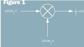
The simplest intermodulation model assumes that two signals are multiplied in a non-linear device as shown in Figure 1.
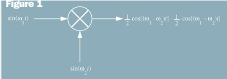
Trigonometric identities tell us that for this simple model, there are two IM products, one with frequency equal to the sum of the original frequencies and the other with frequency equal to the difference of the original frequencies. In practice, IM products are more complex because the non-linearity also creates harmonics of the original frequencies. In general, the frequency of the IM products created by two signals are described mathematically using Equation 1.
Intermodulation products also occur in combinations of three or more frequencies. The number of potential IM products grows rapidly with increasing product order. Simply computing all potential IM products is a non-trivial task if done manually. For example, a small site with just 10 transmitters will have 159,720 combinations of up to three frequencies, 5th harmonic and below.
Multiplication in the time domain is equivalent to convolution in the frequency domain, which means the bandwidth of an IM product is wider than the bandwidth of either of the fundamental interfering signals. The actual spectral shape can be complicated, but a rule of thumb is that the nominal bandwidth of the IM product is equal to the product of the modulation bandwidth of each signal and the order of the IM product. For example, if FM signals ƒ1 and ƒ2 each have a frequency deviation of 3 kHz, the third-order IM product, 2ƒ1 – ƒ2, will have a frequency deviation of 9 kHz.
We also are interested in the power levels of IM signals. Only those products that are 6 dB below the receiver noise floor or stronger will cause noticeable interference. An interfering signal ƒ2 must travel from its source to transmitter ƒ1‘s antenna, down the transmission line and through bandpass cavity filters and ferrite isolators (if any) to reach f1’s final amplifier stage.
At this point, ƒ2 probably will see a poor impedance match and have poor return loss. The small signal that does get through to the final amplifier stage will undergo a mixing loss, and the resulting IM product will have a power level that is strictly less than the power level of ƒ2. The difference between the power level of ƒ2 at transmitter ƒ1 and the power level of the resulting IM product is known as the turn-around loss. Turn-around loss is sometimes referred to as conversion loss, but conversion loss also is equated with mixer loss, which does not include the effects of impedance mismatch that occurs when ƒ2 is offset significantly from ƒ1.
The process for analyzing transmitter IM interference requires that one first gather detailed information on the antenna and transmission line configurations, transmitter turn-around loss, transmitter modulation bandwidths, cavity filters (existing and proposed), ferrite isolators, and receiver bandwidths. If the calculated IM interference is not below receiver threshold, the radio engineer must analyze antenna placement, cavity filter and isolator options to provide additional isolation.
To illustrate this process, consider a simple example of transmitter intermodulation. Our site has two transmitters and one receiver, as shown in Figure 2 on page 38.
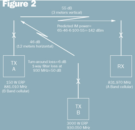
The 930.050 MHz paging transmitter (TX B, ƒ2) causes an IM product to be generated in a cellular base station (TX A, ƒ1 = 881.010 MHz). The IM product, which is shown mathematically in Equation 2, is in the cellular A band (RX, 831.970 MHz).
This product is more than 50 MHz from the TX A frequency, and the transmitter combiner in TX A should provide more than 100 dB of two-way isolation. When the antenna coupling losses, conversion loss, and filter loss are summed, the IM power at the receiver is -142 dBm, which is well below the receiver noise floor and therefore negligible (see Figure 2). Although this example had a happy ending, it illustrates the importance of bandpass filters on transmitters. Without the filter at TX A, the IM product would be -42 dBm and strong enough to wipe out the receiver.
Receiver IM calculations are performed in much the same way as transmitter IM. The mathematical relationships are identical, but the physical mechanism is different. Now the receiver acts as the non-linear device that creates the IM product. Because the IM product is created in the receiver, as opposed to a transmitter, we don’t have the additional isolation from antenna separation between the IM source and the receiver, as we had in the transmitter IM case.
There are two important types of receiver IM. In the first type, IM occurs between strictly external frequencies. The receiver simply acts as the mixing device. This type of IM is routinely measured at the factory for the third order, or 2ƒ1 – ƒ2 case (where ƒ1 and ƒ2 are external frequencies). This test is sometimes called the two-tone intermodulation test. The results of this test can be used to determine the third-order IM rejection capability of the receiver.
In the second case, the receiver also introduces mixing frequencies, usually harmonics of the receiver’s local oscillator, and the IM product is a combination of external and internal frequencies. This type of IM is more difficult to predict because local oscillator frequencies are not always known.
The key to eliminating receiver IM is to reduce the amplitude of interfering signals at the receiver front end. Cavity filters are the preferred tools, but sometimes antenna separation or other forms of antenna isolation are required.
It is important to isolate the source of IM interference before implementing solutions. Filters at the receiver will not solve transmitter intermodulation; similarly, filters at the transmitter will not solve receiver IM.
Probably the most difficult IM problem is passive IM (PIM), which occurs when two or more frequencies mix in a non-active device such as an antenna, loose joint, mating between dissimilar metals, or micro gaps between metal surfaces. Often the culprit is an antenna, especially a transmit antenna because the high currents flowing in the antenna elements make it a more efficient IM generator.
PIM tends to be broadband, and it cannot be corrected with filters or ferrite isolators. Prevention is the best cure for PIM. One should use antennas and connectors with low PIM. DIN connectors are preferred over N connectors. All connectors should use linear materials such as silver, gold and brass. Avoid nickel-plated connectors. Remove unused hardware and transmission lines from the tower and ensure all mechanical connectors and tight and free of corrosion.
Part 2: Common IM problems, real-world examples, and solutions.
Jay Jacobsmeyer is president of Pericle Communications Co., a consulting engineering firm located in Colorado Springs, Colo. He holds bachelor’s and master’s degrees in electrical engineering from Virginia Tech and Cornell University, respectively, and has more than 25 years experience as a radio frequency engineer.