When measurements aren’t feasible
In the absence of drive test measurements, one of the first steps in designing a new land mobile radio system is to model coverage from prospective sites and, through trial and error, find the smallest number of sites that meets the coverage requirement. Alternatively, one may start with a fixed budget and design for the best overall coverage the budget allows.
Before we jump into the morass of propagation models, let’s make it clear that we are interested only in models for land mobile radio propagation at frequencies greater than 30 MHz. This means that models for point-to-point microwave, tropospheric scatter, satellite, AM groundwave and HF skywave are outside the scope of this discussion.
The land mobile radio channel is rarely line-of-sight, and the received signal is the sum of many reflected and diffracted signals. “Multipath fading” describes the time-varying amplitude and phase that characterize the composite signal at the receiver. Because mobile radio receivers are designed to operate in multipath fading mode with a minimum mean amplitude, we are more interested in modeling the mean signal, not the rapid fluctuations caused by fading.
The mean signal amplitude is a function of many factors, including free space loss, terrain loss and clutter loss. At the frequencies used for land mobile radio, we can usually ignore losses due to precipitation and atmospheric absorption.
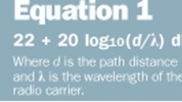
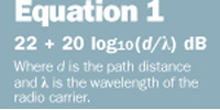
Most propagation models assume that the minimum loss is free space loss. (See Equation 1.) Other losses are added to the free space loss to estimate the total path loss. This assumption normally is sound, but one exception is the so-called waveguide effect in urban areas, where tall buildings on either side of the street act as a waveguide resulting in a path loss that actually is less than free space loss.
Free space loss is easy to compute, so the real problem is to predict the losses due to terrain and clutter. Let’s first address each of these losses and then examine some popular computer models used to predict them.
Terrain loss and digital terrain databases
Terrain loss is primarily diffraction loss, which most models estimate using principles of ray optics. Engineers working at the National Bureau of Standards did much of the work in this area in the late 1950s and early 1960s. The definitive reference for this topic is NBS Technical Note 101, published in 1967. The model described by this note includes the geometry of diffraction as well as the roundness of the obstacle. More advanced models also use the conductivity of the soil, if it is known.
NBS Technical Note 101 does a good job of predicting diffraction loss over isolated obstacles; however, obstacles often appear back-to-back, and simply summing the loss from all obstacles results in an overly conservative prediction. A popular method for sorting out the best way to treat multiple obstacles is the Epstein-Peterson method, which is well-suited for computer models that use digital terrain databases.
A computerized diffraction model is of little use without a digital terrain database. There are several from which to choose — some very coarse and others very fine. In the U.S., the earliest digital terrain databases were the National Geophysical Data Center (NGDC) 30-arc-second and 3-arc-second databases. One pitfall of these databases is that both are taken from the same coarse maps. In other words, the 3-second database is simply a more finely sampled version of the 30-second database. In mountainous terrain, large elevation errors from these databases are likely to occur.
In the early days of personal computers, better-quality terrain data were not available, and even if it were, a sampling finer than 3 arc seconds resulted in unwieldy databases and painfully slow computing. Over the last 10 years, much more accurate terrain data have became available in the form of the 30-meter terrain database, which is extracted from the 1:24,000 scale, 7.5 minute “quad” maps popular with hikers. Modern propagation studies should be done with the 30-meter database or its equivalent, if at all possible.
Clutter loss
Clutter loss falls into two categories: foliage and man-made. Foliage loss is computed from a database of loss factors that are a function of both radio frequency and the type of foliage. Man-made clutter includes buildings, vehicles and bridges. Man-made clutter loss usually is calculated from a clutter database, which applies a clutter category to individual tiles (cells) in the geographical area under study.
Typical clutter categories include dense urban, urban, suburban, industrial, agricultural and rural. A common approach is to apply a single clutter loss factor corresponding to the tile of interest, regardless of the antenna height of the base station/repeater site. This relatively crude model can result in inaccuracies because it is not a function of antenna look angle. The steeper the look angle, the smaller the clutter loss and the shallower the look angle, the greater the clutter loss.
There are dozens of computer propagation models, but we will examine just two of the most popular: path loss slope and Okumura-Hata.
Path loss slope
The path loss slope is the exponent applied to the path distance. Free space loss has an exponent of 2 because received power is proportional to the inverse of distance squared. In the classic land mobile radio model, the theoretical path loss exponent is 4. Because radio engineers prefer to work in logarithms, the path loss exponent commonly is referred to as the path loss slope, with an exponent of 2 equal to a slope of 20 (20 dB per decade).
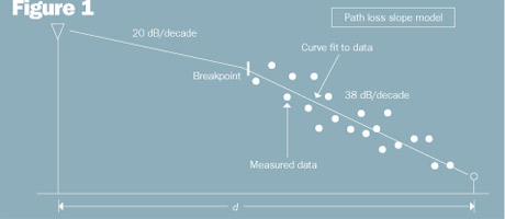
In the cellular radio industry, it is common to fit drive test data to the slope of a straight line (on a log scale) and to use this model for network planning. A common variation of the path loss slope model is the two-slope breakpoint model where a slope of 20 is used from the cell site antenna to the height of the first clutter (assuming the cell site antenna is above clutter). Then, a curve-fitted slope is used from that point to the mobile radio. This concept is illustrated in Figure 1, where the calculated path loss slope after the breakpoint is 38 dB per decade.
Why would a wireless operator use such a crude model when more sophisticated models are available? The reason lies with the relatively poor accuracy of propagation models. Because most of the path loss in cellular radio networks is due to clutter and clutter databases are necessarily crude, it is nearly impossible to predict signal level with accuracy better than +/- 6 dB (standard deviation). In other words, it makes no sense to measure with a micrometer if you are going to cut with a chain saw.
Okumura-Hata
Most land mobile radio propagation models use some variation of Okumura-Hata. (Other popular models include Longley-Rice — often used by the FCC — TIREM, and ray-tracing.) Okumura conducted an extensive set of propagation measurements in the Tokyo metropolitan area in the late 1960s. From these measurements he developed a set of curves giving the median attenuation relative to free space in an urban area over quasi-smooth terrain.
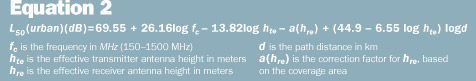
In 1980, Hata published an extension to Okumura’s model that is suitable for computer applications. Okumura-Hata is a statistical model in the sense that actual terrain or clutter is not used in the calculation. Instead, the model computes the path loss as a function of the transmit and receive antenna heights, path distance, radio frequency, and the type of clutter (urban, suburban or open). See Equation 2 for the Okumura-Hata median path loss in urban areas. Correction factors are applied to this basic equation for suburban areas. Common standard deviations between Okumura-Hata predictions and measured path loss are 10-14 dB. For more on the Okumura-Hata equation, see Wireless Communications Principles and Practice by Theodore S. Rappaport.
Jay Jacobsmeyer is president of Pericle Communications Co., a consulting engineering firm in Colorado Springs, Colo. He holds BS and MS degrees in electrical engineering from Virginia Tech and Cornell University, respectively, and has more than 25 years of experience as a radio frequency engineer.